This article is the ninth in a continuing series on the use of decision modeling and optimization techniques for game design. The full list of articles includes:
- Part 1: Introduction (Blogspot) (Gamasutra)
- Part 2: Optimization Basics and Unrolling a Simulation (Blogspot) (Gamasutra)
- Part 3: Allocation and Facility Location Problems (Blogspot) (Gamasutra)
- Part 4: Competitive Balancing Problems (Blogspot) (Gamasutra)
- Part 5: Class Assignment Problems (Blogspot) (Gamasutra)
- Part 6: Parametric Design Techniques (Blogspot) (Gamasutra)
- Part 7: Production Queues (Blogspot) (Gamasutra)
- Part 8: Graph Search (Blogspot) (Gamasutra)
- Part 9: Modular Level Design (Blogspot) (Gamasutra)
The spreadsheet for this article can be downloaded here: link
We've had to put off this instalment of the series for the last few months, as we've been very busy starting up a brand new game studio in Austin.
We're looking forward to announcing more about that in 2014, but in the meantime, we took advantage of Thanksgiving break to finally write up the long-awaited Part 9 of this series. We apologize for the delay and hope to get Part 10 completed by January.
The Story of Pirate Planet
It was a warm day in Austin in April of 2007. As they waited for feedback, the level design team for Pirate Planet on Metroid Prime 3: Corruption grew nervous. They had been working on building Pirate Planet, one of the game's major worlds, for over five months, but for one reason or another -- due to the inevitable delays and re-prioritizations that always occur in game development -- they had never had a chance to show it to Kensuke Tanabe, their supervisor from Nintendo's Software Planning and Development group.Now they were only a scant few months from ship, with precious little time for changes, and Tanabe-san -- a man whose frequent and major design changes were almost as legendary as Miyamoto's -- did not seem pleased.
In fact, he seemed rather disappointed.
Instead of offering his usual feedback, he simply said, "Come back tomorrow. I'll have feedback for you then."
Tanabe-san took a build of the game into his office and shut the door.
When the next day came, the team was stunned. Tanabe's plan was more than an overhaul -- it was a dramatic redesign. Every single room was to be connected to a completely different room than before. The entire world of Pirate Planet was to be completely rearranged, and even many basics such as item pickups were to be moved.
The level design team went through the usual stages that Retro developers experienced when confronted with the often overwhelming feedback from their Nintendo bosses: first, horror at the enormity of the challenge of making so many changes; second, reluctant acquiescence to the fact that they did indeed have to make all the changes listed; and finally, acceptance when they saw the effect of the changes in-game, and realized that nearly all of them were for the better.
The Metroid Prime games benefited enormously from this kind of modular approach to level design, which allowed them to build expensive "rooms" and cheaper "hallways" and separate them with identical doors (which also cleverly masked the loading times as new rooms were streamed in). This gives designers a great deal of flexibility, then, as it allows them to quickly modify the configuration of an entire level. Many games use broadly similar approaches, with The Elder Scrolls: Skyrim being a notable and very successful example.
The configuration of the level, then, can be seen simply as a graph. Each node in the graph is one room, and its connections to other nodes indicate how its various entrances and exits connect to other rooms.
In theory, if we had a formula to tell us whether one graph configuration was "better" than another, we could use that to optimize an entire level, and find the "best" one.
Of course, that's theory. Naturally, if you're an experienced level designer / world-builder, you know that there are far too many factors that go into consideration when building a level to try to build all of these considerations into any kind of neat mathematical formula or an Excel spreadsheet. It's an ongoing, iterative process, with countless considerations based on all of the player's possible paths through the space.
But it's useful to take a look at how you would approach this problem in practice to see what can be done and how you can go about doing it, and what the capabilities and limitations of decision modeling techniques are when we apply them to this sort of problem.
And it's useful to know that there's a tool that can answer part of the problem for us, and suggest possibilities, even if we don't end up using decision modeling to figure out how the rooms are connected.
We can visualize these as similar to the road tiles in the classic board game Carcassonne (playable on Kongregate here):

Assume we have a fixed "level entry" and "level exit," and we need to figure out the best set of rooms that will connect them.

We can place any of our rooms anywhere inside the grid, and we can rotate them arbitrarily. Also, for the sake of simplicity, assume that rooms with 2 exits ("hallways") can be arbitrarily bent or un-bent like a garden hose, so that we can switch any such "hallway" piece between straight and L-shaped as needed.
Your problem is as follows: given the entry and exit points marked above, and assuming you have 9 "2-way" rooms, 4 "3-way" rooms, and one "4-way" room, what's a valid way to place all the rooms in the 5x7 grid above such that each room is used exactly once?
We also paste '0' and '1' values around the outside of the 5x7 grid to indicate which tiles have rooms. The grey tiles on the left and right side indicate the level entrance and exit, respectively.
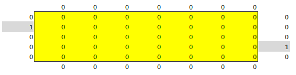
Following the formatting standard we laid out in Part 2, the decision cells are colored yellow to make clear that they are decision variables.
Just below that, we add a second table which counts the number of neighbors of each cell, but only if the cell itself has a nonzero value. This will be our neighbor count. More on that in a moment -- we'll show you the completed table after we solve.
Just to the right of that, we add up all of the things we want to happen when we optimize this table.

Each row of this table indicates a constraint. The "Actual" column determines various things about the actual current characteristics of the decision table or the neighbor count table. The "Desired" column indicates the value we actually require in each case (i.e. the desired value) as stated in the problem statement above (i.e. the values stated in the previous section, "A Sample Problem"). The "Difference" column just subtracts the "Actual" column from the "Desired" column.
Finally, the "Total Difference" cell will be our objective cell. This simply adds up all the values in the "Difference" column. We're trying to minimize that value -- ideally, it should reach 0 to indicate that this problem is "solved."
The first four rows count how many cells of various types exist in the neighbor count table (1-neighbor, 2-neighbor, 3-neighbor, and 4-neighbor cells, respectively), using Excel's COUNTIF() macro. Finally, the last row counts whether there are tiles right next to the entrance and exit.
What else do we need?
Well, in theory, we also need a way to make sure there's a connection between the entrance and the exit.
The constraints above -- telling the solver that we want 0 1-neighbor tiles, 9 2-neighbor tiles, 4 3-neighbor tiles, and 1 4-neighbor tile -- should ensure that we end up with the right number of tiles and that everything is connected in a way that's valid.
If you think about it, though, it should be clear the guarantee of connectivity does not guarantee that there will be an actual path between the entry and the exit. It's possible that individual clusters could form near the entry and exit points, or that there could be separate pieces floating off in the corner, not connected to anything else -- for example, you could get 4 "L-shaped" 2-way tiles in a small square, each connected to two others but none of them connected to the rest of the level.
However, we'll put off dealing with this problem -- proving reachability is overkill for this particular problem, when the fact is, it will probably be fine when we solve it, and if it isn't fully connected as we expect, we can just solve it again to get a new answer.
Finally, we run Excel Solver.

Note how simple this is. We simply set it to minimize the objective cell, then specify the yellow decision cells as the variable cells and add constraints that they must be integers between 0 and 1. We select the Evolutionary method and press Solve!

Note that we've enabled the "conditional formatting" feature in Excel to color the second table -- the one that counts the number of neighbors. As you can see, each cell properly counts how many neighbors it has (if you include the 'entry' and 'exit' cells just outside the table), and there are exactly 9 2-neighbor cells, 4 3-neighbor cells, and one 4-neighbor cells, which is exactly what we wanted.
Problem solved! With just a tiny amount of work, we've gotten Solver to figure out a whole new level configuration for us based on our specifications. We can even run Solver several times with different random seed values to see which level configurations it suggests, and from there, figure out which of those configurations seem to work best.
In terms of Carcassonne tiles, our level would look like this:

We can then use Solver to quickly spit out suggestions for alternate room configurations. For example, if we want to generate a layout with 10 2-neighbor tiles, 6 3-neighbor tiles, and 2 4-neighbor tiles, we could just plug those numbers into our constraint table and re-run Solver to get something like this:


However, with a little work, we could also adapt this to a different, non-orthogonal representation, such as the graph-based representation we used in Part 8. We could also limit ourselves to swapping compatible rooms within an arbitrary fixed configuration, and use that approach to find the best configuration of rooms within a game level without changing the overall layout.
In any event, the fact that it was so easy for us to build this example should tell us something. There are clearly a vast number of ways to apply this approach; if we can only find a useful fitness function for the right configuration of rooms, it becomes almost trivial to apply that to many types of level recombination problems.
Stay tuned for Part 10, due sometime in the next few months, when we'll wrap up our discussion of decision modeling and discuss some very important big-picture issues.
-Paul Tozour
This article was edited by Professor Christopher Thomas Ryan, Assistant Professor of Operations Management at the University of Chicago Booth School of Business.
In theory, if we had a formula to tell us whether one graph configuration was "better" than another, we could use that to optimize an entire level, and find the "best" one.
Of course, that's theory. Naturally, if you're an experienced level designer / world-builder, you know that there are far too many factors that go into consideration when building a level to try to build all of these considerations into any kind of neat mathematical formula or an Excel spreadsheet. It's an ongoing, iterative process, with countless considerations based on all of the player's possible paths through the space.
But it's useful to take a look at how you would approach this problem in practice to see what can be done and how you can go about doing it, and what the capabilities and limitations of decision modeling techniques are when we apply them to this sort of problem.
And it's useful to know that there's a tool that can answer part of the problem for us, and suggest possibilities, even if we don't end up using decision modeling to figure out how the rooms are connected.
A Sample Problem
Suppose for a moment that our game is based on a reconfigurable room system, just like the Metroid Prime games. Assume that we have various types of rooms that all fit within a square grid. We have pre-built rooms that connect 2 neighboring rooms ("L"-shaped or straight line), rooms that connect 3 other rooms ("T"-shaped), and rooms that connect 4 neighbors ("+"-shaped).We can visualize these as similar to the road tiles in the classic board game Carcassonne (playable on Kongregate here):
Assume we have a fixed "level entry" and "level exit," and we need to figure out the best set of rooms that will connect them.
We can place any of our rooms anywhere inside the grid, and we can rotate them arbitrarily. Also, for the sake of simplicity, assume that rooms with 2 exits ("hallways") can be arbitrarily bent or un-bent like a garden hose, so that we can switch any such "hallway" piece between straight and L-shaped as needed.
Your problem is as follows: given the entry and exit points marked above, and assuming you have 9 "2-way" rooms, 4 "3-way" rooms, and one "4-way" room, what's a valid way to place all the rooms in the 5x7 grid above such that each room is used exactly once?
Optimizing Connectivity
We'll begin by using the cells in the 5x7 grid as our decision cells. Each cell will hold either a '0' or a '1' -- a '0' to indicate that there's no room in the cell, and a '1' to indicate the presence of a room.We also paste '0' and '1' values around the outside of the 5x7 grid to indicate which tiles have rooms. The grey tiles on the left and right side indicate the level entrance and exit, respectively.
Following the formatting standard we laid out in Part 2, the decision cells are colored yellow to make clear that they are decision variables.
Just below that, we add a second table which counts the number of neighbors of each cell, but only if the cell itself has a nonzero value. This will be our neighbor count. More on that in a moment -- we'll show you the completed table after we solve.
Just to the right of that, we add up all of the things we want to happen when we optimize this table.
Each row of this table indicates a constraint. The "Actual" column determines various things about the actual current characteristics of the decision table or the neighbor count table. The "Desired" column indicates the value we actually require in each case (i.e. the desired value) as stated in the problem statement above (i.e. the values stated in the previous section, "A Sample Problem"). The "Difference" column just subtracts the "Actual" column from the "Desired" column.
Finally, the "Total Difference" cell will be our objective cell. This simply adds up all the values in the "Difference" column. We're trying to minimize that value -- ideally, it should reach 0 to indicate that this problem is "solved."
The first four rows count how many cells of various types exist in the neighbor count table (1-neighbor, 2-neighbor, 3-neighbor, and 4-neighbor cells, respectively), using Excel's COUNTIF() macro. Finally, the last row counts whether there are tiles right next to the entrance and exit.
What else do we need?
Well, in theory, we also need a way to make sure there's a connection between the entrance and the exit.
The constraints above -- telling the solver that we want 0 1-neighbor tiles, 9 2-neighbor tiles, 4 3-neighbor tiles, and 1 4-neighbor tile -- should ensure that we end up with the right number of tiles and that everything is connected in a way that's valid.
If you think about it, though, it should be clear the guarantee of connectivity does not guarantee that there will be an actual path between the entry and the exit. It's possible that individual clusters could form near the entry and exit points, or that there could be separate pieces floating off in the corner, not connected to anything else -- for example, you could get 4 "L-shaped" 2-way tiles in a small square, each connected to two others but none of them connected to the rest of the level.
However, we'll put off dealing with this problem -- proving reachability is overkill for this particular problem, when the fact is, it will probably be fine when we solve it, and if it isn't fully connected as we expect, we can just solve it again to get a new answer.
Finally, we run Excel Solver.
Note how simple this is. We simply set it to minimize the objective cell, then specify the yellow decision cells as the variable cells and add constraints that they must be integers between 0 and 1. We select the Evolutionary method and press Solve!
Solved!
After running the Evolutionary solver for a while, you may get something that looks like this:
Note that we've enabled the "conditional formatting" feature in Excel to color the second table -- the one that counts the number of neighbors. As you can see, each cell properly counts how many neighbors it has (if you include the 'entry' and 'exit' cells just outside the table), and there are exactly 9 2-neighbor cells, 4 3-neighbor cells, and one 4-neighbor cells, which is exactly what we wanted.
Problem solved! With just a tiny amount of work, we've gotten Solver to figure out a whole new level configuration for us based on our specifications. We can even run Solver several times with different random seed values to see which level configurations it suggests, and from there, figure out which of those configurations seem to work best.
In terms of Carcassonne tiles, our level would look like this:
We can then use Solver to quickly spit out suggestions for alternate room configurations. For example, if we want to generate a layout with 10 2-neighbor tiles, 6 3-neighbor tiles, and 2 4-neighbor tiles, we could just plug those numbers into our constraint table and re-run Solver to get something like this:
Extending the Example
Now let's say we want to extend the example to include the difficulty level.
Assume that each room has an overall difficulty level that represents how much of a challenge the player will encounter in that room, where '1' represents an easy room, '2' represents a moderately challenging room, and '3' represents a challenge, with a room that contains a boss monster or something like that. So instead of simply using a '1' in our decision table for each cell with a room in it, we'll have a number between 1 and 3 indicating difficulty.
Our first criterion is that we want some variation in difficulty levels. So we'll add a new table where each cell measures the change in difficulty between that cell and any nonzero neighboring cells (or 0 if the corresponding cell in the decision table is 0).

Now we add a cell to our constraint table that measures the average difficulty change -- the first row inside the red box in the modified constraint table shown below. It does this using Excel's AVERAGEIF() function to count the difficulty change from the table above if the corresponding cell in the decision table is nonzero.
Assume that each room has an overall difficulty level that represents how much of a challenge the player will encounter in that room, where '1' represents an easy room, '2' represents a moderately challenging room, and '3' represents a challenge, with a room that contains a boss monster or something like that. So instead of simply using a '1' in our decision table for each cell with a room in it, we'll have a number between 1 and 3 indicating difficulty.
Our first criterion is that we want some variation in difficulty levels. So we'll add a new table where each cell measures the change in difficulty between that cell and any nonzero neighboring cells (or 0 if the corresponding cell in the decision table is 0).
Now we add a cell to our constraint table that measures the average difficulty change -- the first row inside the red box in the modified constraint table shown below. It does this using Excel's AVERAGEIF() function to count the difficulty change from the table above if the corresponding cell in the decision table is nonzero.
The second row in the constraint table tests whether there's one cell in the second-to-last column to the right (column H) with maximum difficulty. This will help us ensure that the maximum difficulty is close to the exit, since the exit is at the rightmost side.
We also add a third row to check if every column in the neighbor cell is nonzero. This will return a value of 1 only if each column of the neighbor count table is nonempty. Since we know that a valid solution must have nonempty columns, this constraint will make it more likely that the generated level is fully connected, and there is a path between the "entry" and "exit" cells. By itself, it's not enough to absolutely guarantee that the level it generates will be properly connected, but it gives us better odds than the previous spreadsheet did.
Finally, we make sure these three rows are added to the "Total Difference" objective cell, and solve. Note that the Solver dialog is exactly the same as before, except that we now constrain the decision table cells to have values between 0 and 3 instead of 0 and 1.
Let it run for a few minutes, and voila!
Our decision table looks almost identical to the last one, except that each decision cell has a difficulty level associated with it, and the average difficulty change is 1.
Conclusion
Of course, this is something of a toy problem. We built a grid-based system simply because that's what we can represent most easily with the grid-based design of Excel, but most component-based level design systems don't lend themselves to this format.However, with a little work, we could also adapt this to a different, non-orthogonal representation, such as the graph-based representation we used in Part 8. We could also limit ourselves to swapping compatible rooms within an arbitrary fixed configuration, and use that approach to find the best configuration of rooms within a game level without changing the overall layout.
In any event, the fact that it was so easy for us to build this example should tell us something. There are clearly a vast number of ways to apply this approach; if we can only find a useful fitness function for the right configuration of rooms, it becomes almost trivial to apply that to many types of level recombination problems.
Stay tuned for Part 10, due sometime in the next few months, when we'll wrap up our discussion of decision modeling and discuss some very important big-picture issues.
-Paul Tozour
This article was edited by Professor Christopher Thomas Ryan, Assistant Professor of Operations Management at the University of Chicago Booth School of Business.
No comments:
Post a Comment
Note: Only a member of this blog may post a comment.